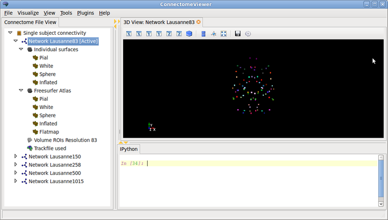
In this tutorial, you will learn about the basic functions you can use to layout your network in 2D or 3D. You will need to open the Single subject connectivity in the ConnectomeViewer. Active the Network Lausanne83 first.
Here the screenshot of what it should look like:
We need to import NumPy and NetworkX:
import numpy as np
import networkx as nx
For each activated network, there exists a DataSourceManager which stores and manipulates the data sources we have, and the RenderManager which deals with visualization aspects of our network.
When you activate the network first, you see the nodes place in 3D based on the center of gravity of the the corresponding Region of Interest of the surfaces. It takes the first surface container (Individual surfaces) and the actual pial surface (Pial) for this computation. Obviously, looking at your networks this way where the node positions convey some spatial meaning might be helpful in some contexts. Often, one is interested more in the topological properties of the networks, and this is where layouting schemes come into play.
In the following, you will learn how to apply the Fruchterman-Reingold force-directed algorithm to position your nodes. We use the algorithm implemented in NetworkX to do the job.
Simply enter in the IPython Shell:
cfile.networks[0].set_weight_key('de_density')
new_positions = nx.layout.spring_layout(cfile.networks[0].graph, dim=3)
The first line sets the de_density edge attribute as default attribute to be taken for the layouting algorithm. The second line takes the actual graph representation of your first network of the connectome file and applies the force-directed algorithm using de_density as weights and stores the positions in a dictionary keyed by the node ids.
The array looks something like this:
In [42]: new_positions
Out[42]: {'n1': array([ 0.03043051,  0.24064767,  0.41777253]),
        'n10': array([ 0.03506719,  0.25608611,  0.40165945]),
        'n11': array([ 0.04404312,  0.2562375 ,  0.39679114]),
        ...
We need to put this positions in a numpy array that is ordered by increasing node it. First, we initialize the array and then loop over the new_positions dictionary to extract the data. Note how you left-strip the n from the key to find the correct indices:
new_pos = np.zeros( shape = (len(new_positions),3) )
for k,v in new_positions.items():
    new_pos[int(k.lstrip('n'))-1,:] = v
Now we are ready to go for updating the visualization. First we update the data using the DataSourceManager, and then the RenderManager is our friend:
cfile.networks[0].datasourcemanager.update_positions(new_pos)
cfile.networks[0].rendermanager.update_graph_visualization()
The output in the 3D View looks like all the nodes got together, building one dense overlapping node. We can disentangle them by updateing the node scaling:
cfile.networks[0].rendermanager.update_node_scale_factor(0.001)
We see there are two outsider nodes which are not connected to any other node (poor Left and Right-Subthalamus with n80 and n39). He makes it hard to navigate the layout nicely. So we just set their value to be in the average position between all other nodes and execute the three last steps from above (updating the source and render manager):
new_pos[38,:] = new_pos[79,:] = np.average(new_pos,axis=0)
Now, everything looks quite good. Let’s see if we can display the edges:
cfile.networks[0].select_all()
That’s it for this tutorial. Of course you can play around now with different graph layouts. If you want to have your layout in 2D, just set the third value to zero in the new_pos array.